Exploring Sentiment Analysis with Nepali Text

Sentiment analysis, a crucial component of natural language processing (NLP), has seen exponential growth in its applications, spanning from understanding customer feedback to social media monitoring. In this blog, I delve into a project that tackled sentiment analysis of Nepali text, illustrating the process, challenges, and achievements along the way.

Background

Nepali, an Indo-Aryan language, is spoken predominantly in Nepal and parts of India. Despite its wide usage, resources for NLP tasks in Nepali are limited compared to languages like English. This project aimed to fill this gap by creating a sentiment analysis model that can accurately classify Nepali sentences into positive, negative, or neutral sentiments.

Data and Preprocessing

The journey began with the dataset, sentiment_analysis_nepali_final.csv, which contained three columns: Unnamed: 0, Sentences, and Sentiment. Each row represented a Nepali sentence and its associated sentiment. The initial preprocessing steps included:

Loading the Data

data = pd.read_csv('/work/sentiment_analysis_nepali_final.csv')

Cleaning

• Dropping unnecessary columns and renaming for clarity.
• Handling null values and duplicates.

df['text'].isnull().sum()
df['labels'].isnull().sum()

Text Preprocessing

• Removal of stopwords in Nepali using the nltk library.
• Tokenization and normalization of the text.

import nltk
nltk.download('stopwords')

from nltk.corpus import stopwords

stopword=set(stopwords.words('nepali'))
X_data=[]
for i in df['text']:
    text=' '.join([word for word in i.split() if word not in stopword])
    X_data.append(text.strip())

Feature Engineering with TF-IDF

The next step was to convert the preprocessed text into numerical features that the model could understand. This was done using Term Frequency-Inverse Document Frequency (TF-IDF), a technique that reflects the importance of words in the corpus.

def tfidf_features(X_train, X_test):
    tfidf_vectorizer = TfidfVectorizer()
    X_train_tfidf = tfidf_vectorizer.fit_transform(X_train)
    X_test_tfidf = tfidf_vectorizer.transform(X_test)
    return X_train_tfidf, X_test_tfidf, tfidf_vectorizer

Model Selection and Parameter Tuning

I chose the Support Vector Machine (SVM) for this task due to its effectiveness in classification problems, especially with high-dimensional data. However, SVM has crucial hyperparameters like C, kernel, and gamma that needed optimization for best performance.

parameters = {'C': [0.01, 0.1, 1, 10, 100], 'kernel': ['rbf', 'poly', 'linear'], 'gamma': ['scale', 'auto']}
grid_search = GridSearchCV(svm.SVC(), parameters, cv=5, scoring='accuracy', verbose=2, n_jobs=-1)
grid_search.fit(X_train_tfidf, y_train)

Parameters for GridSearchCV:

1. estimator:
   • In our case, svm.SVC(). This is the model for which we want to find the best hyperparameters.
2. param_grid:
   • A dictionary specifying the hyperparameters and their possible values. For example, parameters = {'C': [0.01, 0.1, 1, 10, 100], 'kernel': ['rbf'], 'gamma': ['scale', 'auto']}.
3. cv:
   • Stands for cross-validation. cv=5 means you’re using 5-fold cross-validation. This means the data is divided into 5 parts; in each iteration, 4 parts are used for training and 1 for validation.
4. scoring:
   • The metric to evaluate the models. In our case, we are using 'accuracy', so the grid search will select the hyperparameters that achieve the highest accuracy.
5. verbose:
   • Controls the verbosity of the output. verbose=2 means we will get more detailed output (such as the progress of the fits).
6. n_jobs:
   • Specifies the number of jobs to run in parallel. n_jobs=-1 means using all processors.

Parameters of the estimator (SVC in our Case)

1. C:
   • Regularization parameter. The strength of the regularization is inversely proportional to C. Lower values of C lead to stronger regularization(prevent overfitting). Helps to control over-fitting (Overfitting occurs when a model learns the details and noise in the training data to the extent that it negatively impacts the model’s performance).
2. kernel:
   • Specifies the kernel type to be used in the algorithm. we are using 'rbf' which stands for Radial Basis Function, a common choice for non-linear data.
3. gamma:
   • A parameter for non-linear hyperplanes. The higher the gamma value, the more it tries to exactly fit the training data set. scale and auto are two ways of setting this parameter in scikit-learn.

Process

• The GridSearchCV will iterate over all combinations of these parameters (5 values of C, 1 kernel type, and 2 values of gamma), applying 5-fold cross-validation for each combination.
• It will measure the performance using accuracy and finally pick the combination that gives the best result.
• This process helps in finding the optimal hyperparameters for the SVM model for your specific dataset.

This is where the bulk of the time was spent — approximately 6 hours — in finding the best parameters through GridSearchCV, a method that systematically works through multiple combinations of parameter tunes, cross-validating as it goes to determine which tune gives the best performance.

Results

The best parameters were found to be {'C': 10, 'gamma': 'scale', 'kernel': 'rbf'}, achieving a cross-validation score of 0.67 and a test set score of 0.68. These results are promising but also indicate room for improvement.

Then using some Nepali text, I tested the model. Surprisingly, the predictions were mostly accurate.

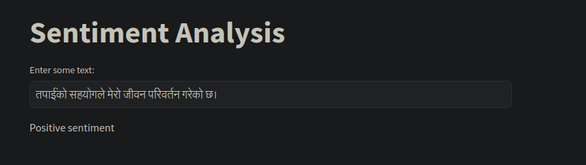
Creating A Web Application

The next step was to create a web application using Streamlit. For this, I exported two files using Pickle.

import pickle
pickle.dump(model, open('sentiment_model.pkl', 'wb'))
pickle.dump(tfidf_vectorizer, open('tfidf_vectorizer.pkl','wb'))

Then using those files, I created the app.

You can find the full code on github.

The dataset is from Kaggle and the article on the medium was helpful for this project.

What More Can Be Done for Better Accuracy?

1. Enhanced Data Preprocessing:
   • More advanced techniques for text normalization and dealing with colloquialisms in Nepali.
   • Augmenting data through techniques like synonym replacement.
2. Experimenting with Different Models:
   • Trying out ensemble models or deep learning approaches like LSTM or Transformers.
3. Hyperparameter Tuning:
   • Further refinement of SVM parameters or exploring other algorithms and their optimal settings.
4. Incorporating Contextual Information:
   • Using pre-trained models that understand the context better, like BERT-based models for Nepali.
5. Error Analysis:
   • Diving deeper into the misclassified examples to understand where the model is faltering and why.

Conclusion

This project showcased the intricacies of sentiment analysis, especially when dealing with a less-resourced language like Nepali. The journey from data preprocessing to hyperparameter tuning was arduous, consuming around 6 hours just for parameter optimization.

Yet, the results were promising, opening doors to more refined techniques and models that can push the accuracy even further. As the field of NLP grows, the horizon for languages like Nepali expands, bringing a more robust and nuanced understanding to the world of sentiment analysis.